Notes on Semi-Streaming Matching

Recently, Sepehr Assadi, Max Jiang, and I presented a proof that the greedy algorithm is optimal in semi-streaming matching. The technical details are on arXiv:

• Semi-Streaming Matching in a Single Pass I: A New Framework for Lower Bounds via Blueprints
• Semi-Streaming Matching in a Single Pass II: Greedy is Optimal

The first paper has been peer reviewed and presented at the STOC 2026 conference. While Max and I independently built a Lean proof for it, the second paper has not been peer reviewed as of the time of writing, which is the usual expectation in the research community before a result is definitively claimed. Note that this blog post and the second paper have not been subjected to the usual scrutiny reserved for formal publications, so this post primarily reflects my personal views and experiences on the problem.

1Intro

Ever since the beginning of the graph streaming subfield [FKM⁺05], a central open question has been whether we can beat the greedy algorithm’s approximation ratio for maximum matching. To explain what that means, and what we proved, let me start with the problem itself.

1.1The Problem

In theoretical CS, a basic question is which problems computers can solve, and which models of computation solve them efficiently. Semi-streaming [FKM⁺05] is a popular and influential model for graph problems: an algorithm reads the input once, front to back, but doesn’t have enough memory to remember all of it. It models a computer that is handed a massive stream of data and must compute something about the whole stream without storing it.

The problem our research focuses on is matching. I’ll assume you’re familiar with graph theory and maximum matching; if not, you can read about it here.

Formally, the edges of an $n$-vertex graph arrive one at a time; a semi-streaming algorithm reads them in a single pass using $\mathcal{O}(n \operatorname{poly}\log n)$ memory, and must output a matching as large as possible.

1.2The Greedy Algorithm

Mathematicians have studied matchings since 1891, when Julius Petersen studied them in a paper that is often considered one of the earliest works in graph theory. There is a well-known algorithm that works in both the classical model of computation and semi-streaming. It has an approximation ratio of $1/2$, which means it always produces a matching at least $1/2$ the size of the true maximum matching. It’s called the greedy algorithm.

1.3Our Results

A central open question has been whether we can beat the greedy algorithm for semi-streaming matching, or more specifically, whether there is an algorithm that has an approximation ratio greater than $1/2$. We show that you can’t: greedy is optimal.

In the first paper, we build a framework for proving lower bounds. If you can construct certain combinatorial objects, which we call blueprints, then no algorithm can beat a corresponding approximation ratio, and the better the blueprint, the smaller that ratio.

In the second paper, we use this framework to prove the tight bound by constructing a blueprint: no single-pass semi-streaming algorithm, even a randomized one, can beat $1/2$. This shows greedy is optimal and settles the question.

2The Idea

Up to our papers, every impossibility result for this problem used an extensively studied graph family from combinatorics called Ruzsa-Szemerédi graphs (RS graphs). We define a new class of graphs, extended Ruzsa-Szemerédi graphs (ERS graphs).

2.1ERS Graphs

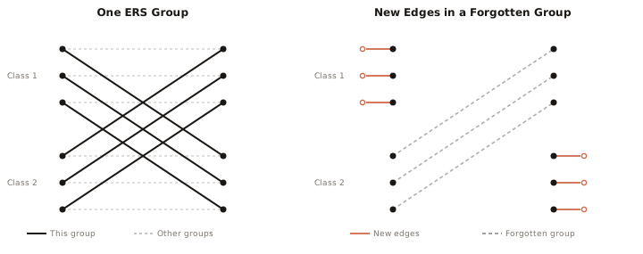
An ERS graph is a bipartite graph with a special structure. Its edges can be split into many groups. For each group, we can split the vertices into two classes on the left and two classes on the right, with an almost perfect matching between each of the four pairs of classes on the left and right.

The property that we care about is that if you look at any other group, its edges go between the same class numbers on the left and right. So a group’s own edges can go between different class numbers, but every other group’s edges always join the same class numbers.

Also, there have to be enough groups that the entire graph is too dense to store directly in memory.

2.2Why One ERS Graph Is a Hard Input

Now stream the entire ERS graph to the algorithm. It’s dense, so the algorithm can’t remember all of it and has to throw most of it away.

Because we forgot most of the graph, there is at least one group, say group $i$, where we forgot most of the edges. Now stream some more edges: for each vertex in the first class on the left and the second class on the right, add an edge to a fresh outside vertex.

The best matching is now the one between the second class on the left and the first class on the right, together with the new edges. But the algorithm forgot most of the edges in this group, so once it sees the new edges, the best it can do is take the new edges. The other groups can’t help. Their edges join the same class numbers on the left and the right, so one endpoint of every such edge already touches a new edge, and there is no reason not to take that new edge, since its only other endpoint is a fresh outside vertex.

This construction is essentially the result of [GKK12], which showed no semi-streaming algorithm can beat $2/3$.

2.3The Ban Constraint

Look again at the edges we added to outside vertices. Every class appears on both the left and the right. And in fact, to keep the streaming algorithm from using edges in other groups, we have to match either the left or the right to outside vertices for each class.

If we match a class out, we can’t use it in the true maximum matching either. So we have to decide on a set of edges to take from the ERS graph and a set of classes to match out. For each class, we have to match it out on either the left or the right, which just means the set of edges we take from the ERS graph can’t have two endpoints in the same class on opposite sides. This is exactly the ban constraint in the paper: we can’t use two vertices on the left and the right in the same class.

The approximation ratio is a function of the proportion of the edges we take from the ERS graph; the more we take, the lower the approximation ratio and the stronger the impossibility result.

2.4Blueprints: A Multilayered ERS Graph

An ERS graph’s input is determined by a single number, the group we chose. Blueprints extend this to $P \ge 1$ layers, where we choose more than one group, one for each layer.

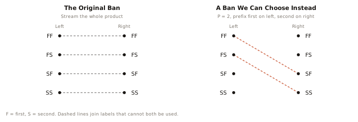
Consider a graph whose left side is the product of $P$ ERS graphs’ left sides and whose right side is the product of the same $P$ ERS graphs’ right sides. In a single ERS graph, every vertex belongs to one of two classes, first or second. In the product, a vertex has one such class in each layer, so it is described by a $P$-tuple of elements from {first, second}, which we call its label. There are $2^P$ labels, and they split each side of the product into $2^P$ classes. We send the product of the $P$ ERS graphs’ edges as input, and as before we still have to choose a set of ERS edges to take, except now each one is a product of $P$ edges, one from each layer.

The ban constraint is the same over this product: for every label, at most one of the left class or the right class with that label can have edges.

There is one more trick beyond streaming the whole product at once. Suppose we want to use an edge between two labels but do not want to force the original ban constraint on ourselves. Fix a layer $p$ between $1$ and $P$, and for each layer $q < p$ fix two classes $x_q$ and $y_q$ in {first, second}, one for the left and one for the right. Now stream only the product edges that, on every layer $q < p$, lie in class $x_q$ on the left and class $y_q$ on the right. The ban constraint changes to match. Instead of disallowing a left label and a right label from both being used whenever they agree on all $P$ layers, we disallow them only when both of the following hold:

1. on every layer $q < p$, the left label has $x_q$ and the right label has $y_q$, and
2. on every layer from $p$ onward, the two labels have the same class.

We stream these inputs one after another, for increasing $p$. This gives us a new degree of freedom: if we want to use a particular edge of the product graph, we can place it in any one of the $P$ inputs, and each choice forces a different ban. Instead of being locked into the single ban of the full product, we have $P$ different bans to choose between for each edge, and we keep whichever one is easiest to satisfy alongside the other edges we want. That freedom is what lets us build blueprints forcing a much smaller approximation ratio.

A blueprint is a finite-sized description of these choices: the number of layers $P$, which ERS edges to take and from which layer, and the classes to match out. A process similar to the one we described turns any blueprint into a hard stream, so proving a tighter impossibility result comes down to finding a blueprint forcing a smaller approximation ratio, which is far more flexible than finding a single ERS graph forcing a smaller ratio. This is exactly the framework we build in the first paper.

3AI Use

3.1Reducing to a Smaller Problem

Some results in theoretical CS, both algorithms and impossibility results, reduce to what is known as a factor-revealing linear program. The idea is to express the worst case of an algorithm as an optimization problem, where a feasible solution is a possible worst-case instance and the optimal value is the approximation ratio. Solving the program reveals the factor. A recent example in matching is the edge-degree constrained subgraph, whose algorithms achieve an approximation ratio determined by a factor-revealing linear program [BK22]. These algorithms give better-than-half protocols for a model of computation closely related to streaming called the $(P+1)$-player communication game of matching, which is exactly the game our $P$-layer blueprints bound from above. Their algorithms are something like duals to our blueprints: a good solution to one implies a bound on the other, the way weak duality relates a linear program to its dual. Strong duality does not hold here, though, so a good solution on one side does not automatically give a matching one on the other.

The usual approach is to reduce your problem to such a program and hand it to a solver like Gurobi. AI has also been used for a similar kind of task before: AlphaEvolve searches for the combinatorial gadgets behind hardness-of-approximation results [NRT25]. I think solving a bounded, self-contained problem like a factor-revealing program is probably much easier for an AI right now than solving the whole problem, perhaps because it misses the big picture, though I can’t really speculate. Our framework instead produces a factor-revealing integer program, which is NP-hard and much harder to solve in general. Throughout our research, we tried solving it with Gurobi, by hand, and with AI, and the final result came from a combination of work by hand and by AI.

3.2Running the AI

The AI acknowledgement in the second paper mentions two independent AI attempts.

The first attempt was with an older Gemini model. We gave it the direct definition of blueprints and asked it to work with them. We did not use any of those results in the final paper.

I was responsible for running the second attempt, a combination of two separate multi-agent runs; in total, the AI ran for many hours, likely days. In the first run, a Fable model, the orchestrator, controlled a set of other Fables. I started it in a directory that contained the first paper and asked it to determine the smallest approximation ratio a blueprint can force. Over time I fed it additional research notes from us. The definitions, theorems, and conjectures its agents produced were stored in the same directory and kept as reference. At each point in time, the orchestrator reviewed the latest results, assigned new tasks, and directed the other agents toward the most promising directions.

The most persistent challenge was keeping the vocabulary under control. Each agent had a tendency to invent its own terminology, so the orchestrator eventually accumulated so many definitions that it stopped making sense. I had to explicitly prompt both the orchestrator and the agents to avoid this, and even then we still ended up with many new definitions.

A second challenge was the orchestrator’s tendency to assign hyper-specific directions. In my opinion this is suboptimal: the amount of reasoning the orchestrator goes through is far less than the reasoning its agents can produce in parallel, so it is better off assigning broader directions and letting the agents explore.

After the Fable run, I spawned a separate Sol agent inside the same directory, which again orchestrated many other Sols. After reading the reports from the Fable agents and the humans, it eventually found the main idea behind the construction we present in our second paper, built from random walks.

3.3Finishing the Proof

After Sol found the idea, we constructed the blueprint presented in the second paper, verified its constraints, and calculated its approximation ratio. When we plugged this into the framework in our first paper, it implied that the greedy algorithm is optimal.